Y-DNA testing has only been around for about 15 years and can tell
us about our direct paternal ancestry.
It is sometimes criticized for only being able to tell us about a small
portion of our genetic history. I think
the critics forget that our mothers have fathers and there are a number of ways
to obtain male test subjects to expand Y results across the entire family
tree. In the last few years, there has
been a brighter spotlight on autosomal testing and its ability to test a larger
portion of our genes. This may have
diverted research attention. Relatively
speaking, y-DNA is still in its infancy and there is much more to be learned. In addition to our deep ancestral origins
dating back over 10,000 years, we should be able to identify our old world
homeland and our nomadic ancestor’s migration routes. It is meaningful to know not only where they
lived, but also when they lived to give us clues to their part in history.

My closest genetic cousins and I share a common
ancestor over 1,100 years ago. With that many years between us, I didn’t
spend a lot of time looking for a common surname. For the last four
years, I’ve been working with y-DNA to determine what can be learned beyond
cousin matches and distant origins. I originally tested with the
Genographic Project and then transferred my results to Family Tree DNA for an
upgrade. In the time since getting my upgrade to 67 markers, I have
received only one match. This is due to my haplotype being somewhat rare
and not a reflection of Family Tree DNA’s ability to provide matches. I learned
that I was part of haplogroup G, from the Caucasus Mountains. I
didn’t learn anything about how the ancestors of my Italian family traveled
from Western Asia to Italy.
I needed to find more cousin matches than the client
base that had tested with FTDNA. Ancestry.com allowed me to enter my
y-DNA markers into their DNA section. I compared my haplotype against the
database at Sorenson Molecular (SMGF.org). I also tried Genebase.com and
any other place I could find. I didn’t locate any cousins. I did
get a good education on what is out there for DNA companies and services.
FTDNA allowed me to transfer my results to Ysearch.org, a free public DNA
matching service that they provide. Ysearch provided much more
flexibility. Where FTDNA would only show me matches with a genetic
distance of seven or less, Ysearch allowed me to select the genetic distance.
Without the genetic distance restrictions, Ysearch showed me hundreds of very
distantly related cousins. I’d rather have distant than none. FTDNA
is not trying to be difficult. They are trying to be realistic and keep
matches within genealogical timeframes. I just needed more.
While not used consistently, one of the best features
of Ysearch is its ability to present the most distant known paternal ancestor
(MDKPA) and their origin. So now, I had cousins and their ancestral
origins. The greater the genetic distance, the closer I got to the
Caucasus Mountains. I mapped my closest cousins and their pushpins
created a line from the Alps to the North Sea, directly along the Rhine River.
This was a pattern. I like patterns. There is usually a
scientific reason for a pattern.
Figure 1 – Mapping Ancestral Origins
I’ve run a few hundred
genetic mapping exercises on the majority of Y haplogroups. The patterns are consistent. Our ancestors traveled along rivers and
coastlines. They skirted mountain ranges
and crossed bodies of water. There is
always a flow to the patterns, but the science and the why were still missing. I’ve always been interested in early Eurasian
history and have tried to associate it to the patterns in the maps that I
generated. Some maps have places and
dates that connect well to notable events.
Other maps raise more questions than answers. Genetic tests and history alone were not
making a complete picture. I needed to
add population genetics, migration models, anthropology and evolutionary
biology to my knowledge base.
Take any two people on the planet, compare their DNA and you can
calculate, approximately, how far back in time their common ancestor lived –
time to most recent common ancestor (TMRCA).
Our ancestors were nomadic and traveled about 25 to 30 km per generation
or roughly 1 km/year on average. If a
common ancestor lived 300 years ago, then that person’s descendants may have
migrated 300 km from the geographic origin of that ancestor. In the figure below, d1 and d2
represent the origins of two known y-DNA genetic records. The circles show the distance their ancestors
may have migrated. The intersections are
the potential locations of their common ancestor. In this case, there are two intersections, a1
and a2. More y-DNA records
are required to figure out which intersection is correct.
Figure 2 – Distance to Most Recent Common Ancestor
(Bilateration)
The genetic analysis that
I have developed is similar to a navigation technique. Radio navigation uses two or more beacons
with known locations and a measurement of the time it takes to receive a signal
from each. The time is converted to a
distance. A current location can then be
identified. In my method, the “beacons”
are the ancestral geographic origins. The
“signal” is the TMRCA, measured in years, converted to a distance by
multiplying the average migration rate – creating a distance to most recent
common ancestor (DMRCA). A location for
the common ancestor can then be figured out by looking at the intersections. Multiple y-DNA records are needed to
determine migration direction and geographic origins of a related set of
genetic cousins. The science is starting
to take shape.
I am G-Z726, which is a subgroup of G-Z725. At Ysearch or on an FTDNA project you may still see an older naming convention - G2a3b. As an example, let’s look
at 18 of my closest genetic cousins – haplogroup G-Z725, (DYS388=13). TMRCA data is generated using Dean McGee’s
Y-Utility. The output is turned into a
phylogenetic tree and the DMRCA is calculated.
Figure 3 - Phylogenetic Tree - G-Z725 Sample
Each distance is used to draw a circle that represents the
migration range of that ancestral line.
My range (MAG) and the range of my next closest cousin on the tree (BAB)
create two intersections on the map. One
point is in Africa and the other is in Eastern Europe.
Figure 4 - Intersection of MAG and BAB
By adding the range of cousin EBE, the correct intersection representing
common ancestor 7 (CA7) is identified.
Pairs of records are mapped to continue the analysis.
Figure 5 - Intersection of BIR and RUF
BIR and RUF are another example and they identify common ancestor
CA3. Each record is added until all
common ancestors are identified.
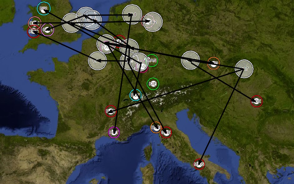
Figure 6 - Common Ancestors Mapped
Connections are drawn based on the phylogenetic tree.
Figure 7 - Phylogenetic Tree Superimposed
Then for simplification, the migration flow is generalized. Based on the phylogenetic analysis, common
ancestor 7 (CA7) is the most distant common ancestor (MDCA) of samples in this
example. The western migration flow has
a slight correlation to the Danube River and the North/South migrations have a
strong correlation to the Rhine River.
Early attempts at direct mapping of genetic data (Fig. 1) gave similar
results based on TMRCA alone. There was
no corroborating evidence of directionality or definitive proof of MDCA.
Figure 8 - Generalized Migration Flow - G-Z725
The new methodology that I have developed
shows ancestral origins and migration direction. I call this method biogeographical
multilateration (BGM). It is the
geographical distribution of y-DNA data based on multiple distance measurements
from reference positions.
This method also has the
potential to identify the location of a DNA sample when the origin is unknown. For
one of my clients, I identified that his paternal ancestor that had immigrated
to the United States may have anglicized their name. The previous name was German and that surname
was found predominantly in central Germany.
Applying biogeographical multilateration to my client’s y-DNA results,
while leaving the origin as an unknown, indicated a continental European origin
within 200km of the city with the highest surname density.
In the referenced paper,
the example haplogroup, I-L22, has an approximate correlation to the
Norse/Viking invasions of Britain and identifies a Frisian coast staging area.
Figure 9 - Generalized Migration Flow - I-L22
We are still in the
infancy of what we can learn from y-DNA.
My BGM analysis has room for refinement.
There is enough science out there to help us. New research is being done at the aggregate
population level. We can apply elements
of that research to the individual level.
Biogeographical multilateration has the potential to fill the gap in our
knowledge between genealogical records and deep haplogroup roots. This new tool can give us old world ancestral
origins, migration flow and historical timeframes.
I needed to learn more
about my DNA and my origins. The big
testing companies haven’t filled the knowledge gaps that exist. They are in the business of providing quality
test results. The analysis and tool
creation is falling on the shoulders of “citizen scientists”. Sometimes, you just have to do it yourself.
Reference:
Maglio, MR (2014) Y-Chromosome
Haplotype Origins via Biogeographical Multilateration (Link)